Visualizing Agent Evaluation Metrics Over Time

A customer service agent tells a user it booked the flight. It didn't book the flight. The agent hit a held-out benchmark during training and passed, so nobody flagged it before launch, and only after deployment did the containment rate settle at a stubborn 45%, far below what the pre-launch numbers had promised. That gap between "passed the benchmark" and "works in production" is the subject of this piece.

A correct final answer says nothing about whether the agent looped three times before landing on that answer, called the wrong tool and quietly recovered, leaked part of its reasoning chain into the response, or wore the user down over several turns before finally getting there. Static, pass/fail scoring answers only one question: did the agent get this specific task right. It cannot show whether the agent keeps getting things right as the traffic, the model, and the tools underneath it keep changing.

Three things in particular slip through a single-snapshot score entirely. Drift is one: a gradual erosion of tool-call accuracy or trajectory quality that accumulates over thousands of turns without ever tripping a hard threshold on a held-out set. Recovery is another, since a benchmark cannot tell you whether the agent genuinely corrected a bad tool call or just papered over the failure in its final output. And then there are failure cascades, where a single wrong intermediate step compounds silently through a multi-step workflow, a pattern that tau-bench's approach of verifying the actual database state at the end of a conversation, rather than trusting the agent's own account of what happened, was specifically built to catch.

None of this is a testing oversight so much as a structural mismatch. Evaluation, as most teams practice it, is built for pre-launch readiness: does the agent clear the bar before it ships? But the real management problem starts after that bar is cleared, when the job becomes keeping the agent behaving correctly across changing real-world traffic, model provider updates, and tool changes it was never benchmarked against. Framed differently, an agent in production is less a shipped artifact and more a living digital product, one that needs the same kind of continuous monitoring any changing system requires. The rest of this piece works through what to track, how to visualize it so temporal patterns are readable, and what to do when a pattern appears on the chart.

The three evaluation layers that time-series visualization must cover

Before any of that visualization work can happen, it helps to be precise about what "agent behavior" even consists of. Agent behavior isn't one signal but three nested layers, and squashing them into a single composite metric destroys the diagnostic resolution needed to act on a temporal pattern once it appears.

The first layer is final-answer evaluation: scoring the last output an agent produces against some expected result. It's a necessary check, useful for regression testing, but insufficient by itself, because a wrong path can still stumble onto a right answer. An agent that takes several unnecessary detours and still lands on the correct number looks identical, at this layer, to one that solved the task cleanly, because a correct final answer tells you nothing about whether the agent looped before answering.

The second layer is trajectory evaluation, which scores the entire sequence of model calls, tool calls, and the arguments passed to each one. This layer captures tool-call accuracy, how many steps were taken relative to the minimum required, whether the agent looped, and whether it recovered from its own mistakes. A correct answer reached in more steps than necessary, with a policy-violating intermediate step buried somewhere in the middle, counts as a failing trajectory even though the final-answer layer would wave it through.

The third layer is per-turn evaluation, which scores the meaning of each individual turn as it happens in production, covering jailbreak attempts, a leaked system prompt, a policy violation, and signs that the user is getting frustrated. None of these register in a status code, a latency measurement, or a token count, so standard logs and traces simply do not see them.

The trap, according to MorphLLM's analysis, is treating the first layer as the whole job. A held-out pass/fail can glow green on a dashboard while the trajectory it scores was a mess and three separate turns drifted off policy. Each layer moves at its own pace, too: final-answer scores shift slowly and reveal broad regressions well suited to a weekly trend line, trajectory metrics such as tool-call accuracy and loop count move faster and surface behavioral drift before the final-answer score ever budges, and per-turn labels are the highest-frequency signal available, often the earliest warning that something is going wrong in live traffic. That layered, differently-paced structure is what a visualization strategy has to be built around, which is the subject of the next section.

How the choice of metric determines what patterns become visible

Choosing the wrong metrics to chart doesn't just produce noise. Choosing the wrong metrics produces a clean, reassuring line on a graph that hides the failure the metrics failed to capture.

MorphLLM's analysis narrows the field to six metrics that carry most of the diagnostic weight over time. Task completion, or success rate, has to be verified against the resulting system or database state rather than the agent's own final text, because an agent that reports success without actually changing anything is invisible to a text-only metric, which is precisely the failure mode tau-bench's DB-state verification was designed to catch. Tool-call accuracy tracks whether the agent picked the right tool and the right arguments on each call, and when plotted over time, a dip here tends to arrive before the final-answer score degrades, making it a genuine early-warning signal rather than a lagging one.

Step and loop count matters because loops are otherwise invisible in an aggregate trace: a twenty-step turn and a three-step turn both return one answer, so only per-step attribution reveals that one of them wandered. Trajectory match, comparing the agent's actual sequence of steps against a reference path, is most useful in agents where a correct path is well-defined and deviations from it are meaningful. Cost and latency need to be attributed per step rather than summed per session, because a hidden twenty-step loop raises cost quietly until someone breaks the total down by step and finds where it went. And for RAG-backed agents, groundedness or faithfulness, whether the claims in an answer are actually supported by what was retrieved, rounds out the list; Ragas metrics like faithfulness, context precision, and answer relevancy are mostly reference-free, though context recall specifically needs a ground-truth reference to compute.

Two further categories belong in the same time-series view even though they sit outside the technical stack. Goal fulfillment metrics, containment rate and completion rate chief among them, are the strongest business-outcome signal available, according to Master of Code's Henrique Gomes, and a containment rate climbing from a weak launch number to something respectable across an optimization sprint tells an ROI story that trajectory metrics alone cannot tell. User satisfaction proxies, CSAT, confusion triggers, one-answer success rate, belong in the same time-series view as technical metrics because satisfaction often degrades before tool-call accuracy does.

The common mistake threading through all of this is tracking cost at the session level and stopping there. A looping agent whose loop count quietly doubles over two weeks will not show up in that aggregate cost chart at all until the billing cycle closes and the invoice arrives as a surprise. The fix is picking metrics granular enough that the pattern has somewhere to show up in the first place, not building a better chart.

Structuring a time-series visualization for readable temporal patterns

Picking the right metrics only solves half the problem. Drift, recovery, and cascades are three genuinely different temporal patterns, and each one needs its own visualization structure; a dashboard built for snapshot inspection will hide all three at once.

Drift needs room to breathe: a long enough time window and a stable baseline to measure against. Plotting task completion rate over rolling seven- or thirty-day windows, set against the baseline established at launch, is what makes a gradual decline visible in a way that any single point-in-time score simply cannot capture. Recovery patterns need a finer time resolution than session-level aggregation allows. A chart that rolls everything up by session will show only that the agent eventually got there; a turn-level sequence view reveals that it called the wrong tool, noticed the failure, and corrected itself on the very next step, a pattern to reinforce, distinct from a masking pattern that looks identical from a distance but signals fragility rather than competence.

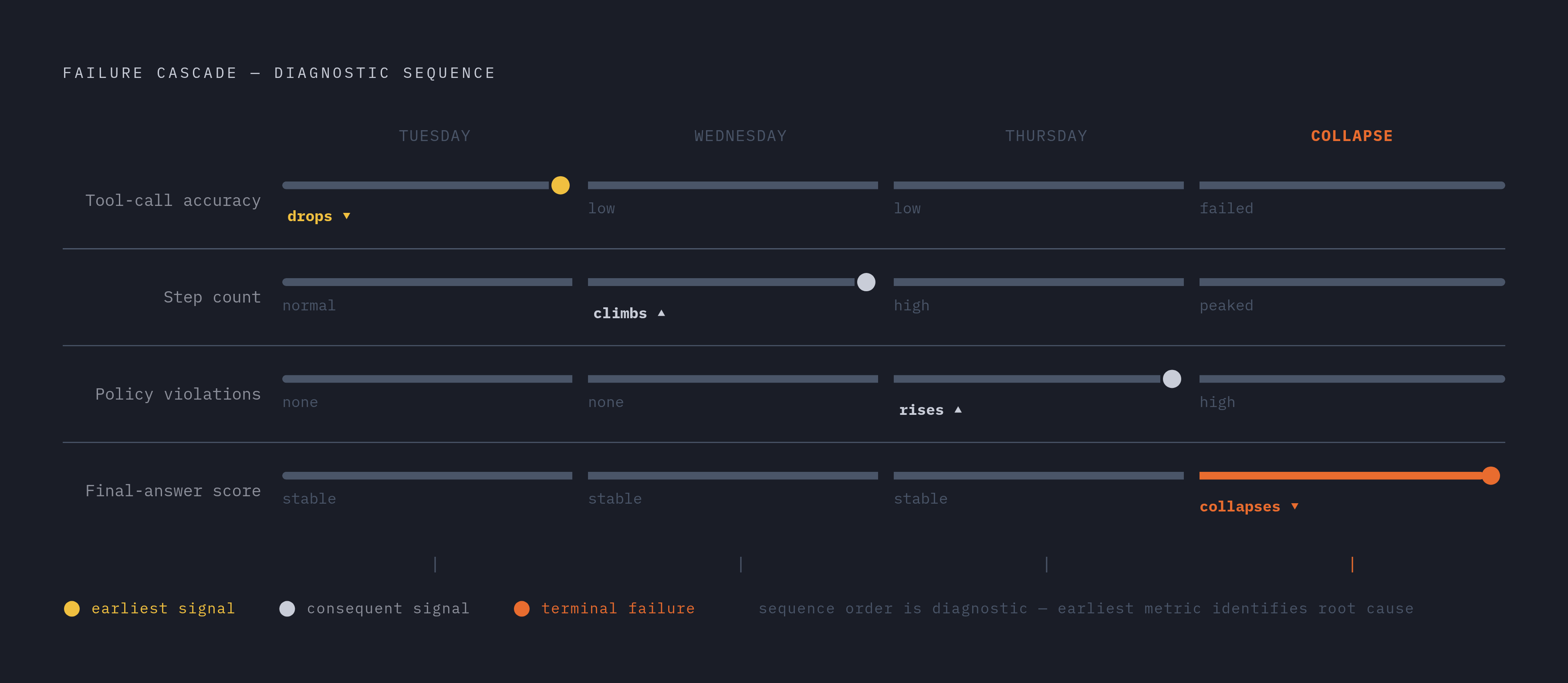
Failure cascades need correlated, multi-metric panels sharing a single time axis. If tool-call accuracy drops on a Tuesday, does step count climb on Wednesday, followed by a final-answer score collapse on Thursday? Separate charts, each metric on its own screen, make that kind of sequence essentially invisible, because nobody is looking at all three at once, while a shared-axis panel puts the sequence right in front of the person reviewing it.

MLflow's approach leans on trace timeline visualization for exactly this reason: trace timelines and per-turn scores are displayed in a UI instead of leaving engineers to dig through raw JSON logs, on the principle that diagnosis should begin with a visual pattern rather than a query someone has to think to write. Its scorer framework, invoked through mlflow.genai.evaluate(), evaluates full execution traces, tool calls, reasoning chains, planning decisions included, so the resulting visualization reflects the agent's actual reasoning loop and not just its inputs and outputs.

Other frameworks solve for different shapes of the same problem. Maxim AI builds custom dashboards aimed at deep behavioral insight and is used by teams including Thoughtful, Mindtickle, and Atomicwork for evaluating multi-agent workflows. LangSmith, built by the LangChain team, is naturally strongest for teams already working in LangGraph, offering comparison-view dashboards for weighing experiments against each other and annotation queues for routing samples to human reviewers. Arize, which started in ML observability before extending into LLM evaluation through Phoenix, brings online monitoring and continuous production evals through its managed platform, Arize AX, a natural fit for teams that already run ML infrastructure and want to fold agent metrics into a time-series view they've already built. None of these is a strict upgrade over the others. Each reflects a different starting point, multi-agent orchestration or existing ML observability stacks among them, and the right choice depends on which of those a team already has in place.

Offline evaluation catches regressions; online evaluation catches what offline cannot anticipate

Offline and online evaluation aren't rivals competing for the same job. They answer two different questions, and a visualization strategy that only covers one of them has a blind spot in a very predictable direction.

Offline evaluation is for reproducible regression detection against known cases. It belongs in continuous integration, running on every prompt change or code change, and its answer to a fairly narrow question, did the agent get worse on yesterday's tasks, is one it can give reliably. What it cannot do is anticipate inputs that don't exist in the dataset yet, catch a multi-turn conversation that drifts somewhere the test set never modeled, reproduce a tool failure that only occurs against a live system, or account for the long tail of user behavior that no held-out set assembled last month could have predicted.

Online evaluation is what closes that gap, by scoring real traffic as it arrives, and it matters for time-series visualization specifically because production traffic is where drift originates, where novel failure modes first appear, and where frustrated users actually show up. There's a real constraint on how this gets built, though. MorphLLM's analysis points out that LLM-as-judge scoring is too slow and too expensive to run against every single production turn, so a per-turn classifier running in a single forward pass, well under 100 milliseconds, becomes the practical requirement for feeding a live time-series view continuously.

The two modes connect through a feedback loop rather than running in isolation. Maxim AI's Data Engine takes production failures and converts them into evaluation datasets, which then power pre-deployment simulation, a mechanism that makes the offline test suite steadily more representative of what real traffic actually looks like. MLflow frames the same idea as a core design requirement: production traces should convert into evaluation datasets, quality regressions should surface as signals someone can act on, and the distance between finding a problem in production and confirming a fix in staging should stay short.

One piece of this still lags behind the ambition. Acting on a temporal pattern, once it's visible on a chart, often requires reconstructing why a metric moved at a particular point in time, and that kind of replay depends on infrastructure most workflow platforms don't yet provide, since none has settled on a portable, end-to-end execution contract with genuine replay support built in. Seeing the pattern is easier than reconstructing the exact chain of events behind it, which is the half current tooling hasn't fully solved.

The three temporal patterns worth acting on

A metric moving on a chart isn't inherently useful information. What matters is knowing which movement demands an immediate page, which warrants a scheduled investigation, and which is just the ordinary noise of a non-deterministic system, because confusing these three wastes engineering time on one end and misses a genuine failure on the other.

Gradual drift is the first pattern: task completion rate or tool-call accuracy sliding downward slowly over days or weeks with no deployment event sitting behind it. The usual suspects are a model provider update nobody flagged, an upstream API that changed its contract quietly, or user behavior migrating away from whatever distribution the agent was originally trained against. The signal to watch for is a trend line pulling away from its rolling baseline rather than any sudden cliff, and the correct response is trajectory-level analysis to pin down exactly which tool calls or step sequences are the ones degrading.

Recovery signature is the second: a metric dips and then climbs back to baseline within minutes or hours. Two very different things can produce that identical shape on a chart. A healthy recovery looks like the agent detecting a failed tool call and retrying correctly, while a masking pattern shows a spike in step count riding alongside a return to normal-looking final-answer scores: the agent got there anyway but took a much longer, messier road to do it. Telling the two apart requires the visualization to show step count and trajectory match right next to the success rate, because a masking pattern is a real cost and reliability risk that a success metric showing normal values does not reveal.

Failure cascade is the third, and the most consequential to catch early: a correlated drop moving across multiple metrics in sequence, tool-call accuracy falling first, step count climbing next, per-turn policy violations rising after that, and finally the collapse of the final-answer score itself. The order in which that sequence unfolds is itself diagnostic. A cascade that starts with tool-call accuracy generally points back to a tool integration or a prompt change, while one that starts with per-turn policy violations more often points to a shift in incoming traffic or an emerging prompt injection pattern, so the direction the cascade travels tells you where to start looking.

Master of Code's documentation of the containment-rate trajectory is the clearest illustration of why this matters beyond engineering. Agents launching with a weak containment rate and climbing to 60% or higher after a focused modification sprint give a temporal arc that, plotted against the specific interventions that produced it, becomes the actual evidence base for deciding on further investment. Not every wiggle in a chart deserves a response, either. Per-turn policy violation spikes and a collapsing trajectory match warrant an immediate one, slow drift in step efficiency warrants a scheduled look, and final-answer scores bouncing around inside a normal variance band are just the expected noise of a system that was never going to be perfectly deterministic in the first place. Knowing the cascade's direction is what turns a chart from a curiosity into an actual lead, and that lead runs straight into a question about infrastructure: can the runtime even produce data granular enough to show it?

Why the runtime executing the agent determines what temporal data you can collect

All of the visualization design in the world doesn't help if the runtime underneath the agent can't actually produce clean, granular data to visualize. The resolution and continuity of any temporal metric depend directly on whether the runtime can maintain state, surface a per-step trace, and run long tasks without losing context along the way, capabilities that generic containers were never built to provide.

Per-step trace attribution is the first requirement. Cost and latency need to be measured per step rather than summed across an entire session, because a runtime that only surfaces session-level telemetry makes loop detection and step-count trending impossible before the analysis even starts, and stateful execution across interruptions matters too: an agent suspended mid-task and resumed later needs to present a continuous trace when it comes back, and a runtime without durable state produces gaps in that trace that look like a metric drop on a chart when they are really an artifact of the infrastructure underneath.

Isolation is the third piece, and it's easy to get backwards. The New Stack's sandbox performance analysis found that slow sandbox command-execution speed can add seconds to what should be millisecond tool calls, distorting latency metrics and breaking the agent's reasoning chain. Infrastructure latency and agent latency have to be separable in the trace, or the chart ends up measuring the sandbox instead of the agent. The architecture of that isolation matters for data integrity too: microVM-based approaches such as Firecracker or Kata Containers give each workload its own dedicated kernel, so one agent's resource contention cannot bleed into another agent's latency numbers, a contamination problem that shared-kernel container environments are structurally prone to.

Purpose-built agent runtimes, as distinct from generic containers or developer sandboxes retrofitted for AI workloads, are designed around these requirements: fast provisioning that does not add measurement noise, stateful execution that preserves trace continuity, and isolation that keeps each agent's telemetry clean. Northflank, confirmed in 2026, offers a full stack covering sandboxes, persistent services, background workers, and databases under a single control plane. The choice of runtime, in other words, isn't a detail to settle after the evaluation strategy is built. It determines whether drift, recovery, and cascade show up cleanly enough on a chart to argue about in the first place.